

Bob’s Imaging Fundamentals #3: Pseudocolor and LUTs
Background: Making the Most of Monochrome
Many types of imaging, from x-ray to infrared, produce monochrome images that need to be post-processed to make the information more useful and interesting. It could be an art project with toy robots or scientific imaging that uses multiple data sets from across the spectrum to make those lovely NASA photos we know and love.
How to Color With Look-Up-Tables
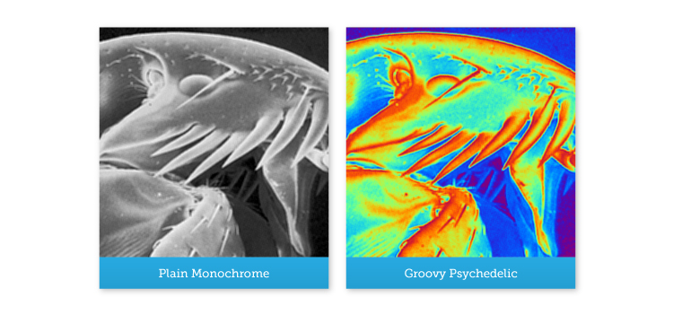
This article builds on the topic of Look-Up-Tables by introducing a technique called ‘pseudo-coloring’. If you are new to the subject of Look-Up-Tables, just remember to call them ‘LUTs’ at Machine Vision parties, or people will have you pegged for a newbie faster than you can say ‘Image Processing’ (you can also follow the links at the end of this article for a bit of an introduction). Now, let’s see how I got Mr. Bug to go from plain monochrome, to groovy psychedelic:
The basic principle of pseudo-coloring is to take a monochrome image and assign each gray value a color. Obviously, to do this we must create a color image and there are a couple of different types of color image we could use. However, I am going to stick to the one most of you already know, the 24-bit ‘true-color’ image format. Now, in our example, we will be going from an 8-bit monochrome image (256 possible gray levels) to a color image having no more than 256 distinct colors. For those of you whose eyes have just glazed over, here is the difference between 8-bit monochrome images and 24-bit color images:
Standard Monochrome:
- 8 bits per pixel (each pixel consists of an 8 bit numerical value)
- Allows 256 different gray levels (28 = 2x2x2x2x2x2x2x2 = 256)
True-Color RGB:
- Each pixel is represented by three 8 bit color bytes R, G and B: 8-bits of Red, 8-bits of Green and 8-bits of Blue i.e., 3 x 8 bits = 24 bits.
- 24 bits allows for 16,777,216 different colors (224 = 2x2x2x2x… = 16,777,216)
“Now wait a minute! Didn’t he just say there wouldn’t be more than 256 distinct colors!?!” Give the smarty-pants in the back row a t-shirt! That’s right, although each pixel in a true color image can have any of 16 million possible colors; our source image only has 256 distinct gray values. So, for our output image, we are only going to use 256 colors out of a possible 16 million. The tough part is deciding which 256 colors to use!
The first step in going from 8 bits to 24 bits is to build three Look-Up-Tables, one for Red, one for Green and one for Blue. The next step is to fill each LUT with a slightly different list of numbers. This can be accomplished in a whole bunch of different ways, but I kind’ a like the results you get with circular functions (see “Graph of Color LUTs”):
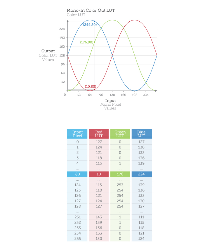
Why does each LUT have to have slightly different values? Because in an RGB image, if all three color bytes are the same, you end up with a monochrome ‘color’ instead of a color ‘color’ e.g., R=128, G=128, B=128 gives you middle of the road gray and similarly, 255, 255, 255 gives you white.
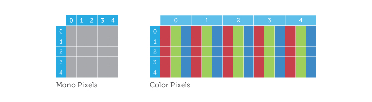
So now we’ve got our original monochrome image, and one LUT for each color component. The final step is to go through our image one pixel at a time and for each pixel determine the corresponding R, G and B color values. For example, let’s say we run into a input-pixel whose value is ‘80’, in this case the corresponding output-pixel’s value would be R=10, G=176, B=244 (see graph and table above). Now remember, we are converting an 8 bit-per-pixel monochrome image into a 24 bit-per-pixel color image, so it’s normal that your output image size is three times larger because each pixel now needs three bytes to define a color instead of just one byte to define a luminance:
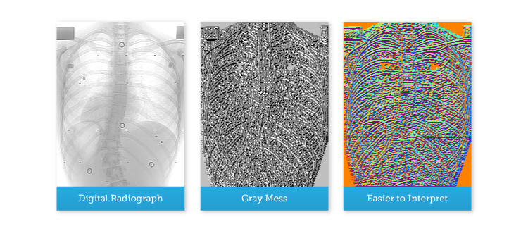
At this point some of you may be wondering why go through all the trouble? The image looked just fine in black and white, right? Well, aside from making it easier to see details that may not be visible in monochrome (i.e. the dark parts), pseudo-coloring did not really add much to the interpretation of this particular image. However, in some applications like X-Ray baggage screening for airport security, adding color to an image can make it much easier to distinguish between different objects. Another use of pseudo-coloring is simply to enhance visual interpretation. For example, let’s say you’ve developed some really cool processing for digital chest radiographs, but in monochrome, the image just looks like a gray mess:
Note: At no time were any bugs forced to take drugs during the production of this article.
Further Reading:
About this article: Bob’s Imaging Fundamentals is an article series based on the work of Bob Howison. Originally titled Bob’s Brain Snacks, these articles were intended to help employees and partners get up to speed with the fundamental concepts of image processing. They became such a popular reference that we’ve decided to bring them to the Possibility Hub. As technology goes further, faster, and new industries discover the power of digital imaging, it’s important to remember the basics.
Bob’s Brain Snacks are recommended for anyone interested in learning about imaging technology. Sharpen your mind and try one!