

Advances in AI for Industrial Inspection
The manufacturing industry is being turned on its head as AI and deep learning turn quality inspection inside-out.
The manufacturing industry is being turned on its head as AI, and deep learning transforms the way we create goods and how quality inspection is employed. The combination of software, new deep learning techniques, power of parallel processing, and ease-of-use tools is at the core of this transformation.
While traditional image-processing software relies on task-specific algorithms, deep learning software uses a multilayer network implementing pre-trained or user-trained algorithms to recognize good and bad images or regions. Traditionally, hundreds, or even thousands, of high-quality, manually classified images were required to train the system and create a model that classifies objects with a high degree of predictability. Just gathering this type of dataset has proven to be an obstacle, hindering deep learning adoption into mainstream manufacturing environments.
New technology advancements are making it easier for manufacturers to embrace deep learning as part of the inspection process. Today, we train deep learning systems with fewer bad images or even none. While deep learning software for machine vision has been around for more than a decade, it is now becoming more user-friendly and practical. As a result, manufacturers are moving from experimenting with deep learning software to implementing it.
Deep Learning vs. Traditional Methods
Deep learning is ideal for tasks that are difficult to achieve with traditional image processing methods. Typical environments that are suitable for deep learning are those where there is a lot of variables, such as lighting, noise, shape, color, and texture. For example, in food inspection, no two loaves of bread are exactly alike. Each loaf has the same ingredients, and each weighs the same amount, but the shape, color, and texture may be slightly different but still within the range of normality.
Another example may be the ripeness of an apple. Ripeness could mean color, softness, or texture; however, there is a range of possibilities where an apple is considered ripe. It is in these types of environments where deep learning shines. Other examples are inspecting the surface finish quality, confirming the presence of multiple items in a kit, detecting foreign objects, and more, to ensure quality throughout the assembly process.
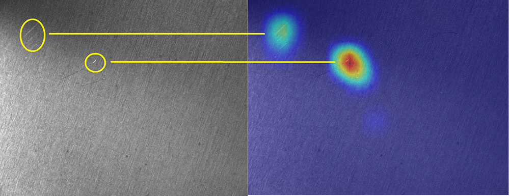
A practical example showing the strength of deep learning is scratch inspection on textured surfaces like metal. Some of those scratches are less bright, and their contrast is in the same order of magnitude than that of the textured background itself. Traditional techniques usually fail to locate these types of defects reliably, especially when the shape, brightness, and contrast vary from sample to sample. Figure 1 illustrate scratches inspection on metal sheets. Defects are clearly shown via a heatmap which is a pseudo-color image highlighting the pixels at the location of the defect.
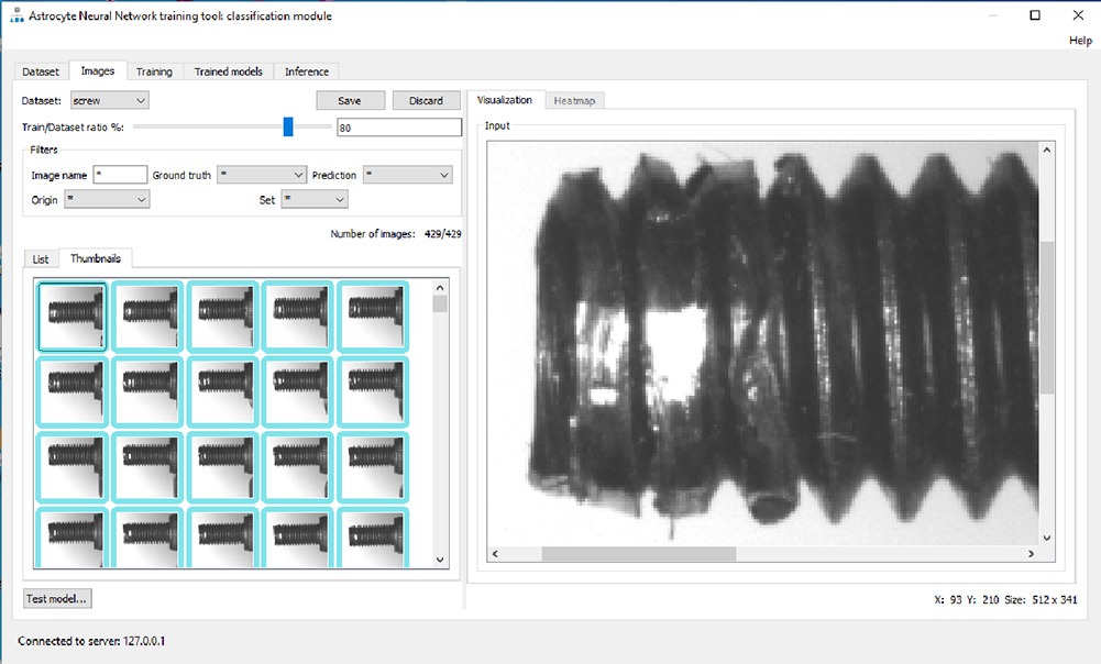
Another example of defect inspection is the ability to classify a complex part as being good or bad as. For instance metal screws are objects presenting a high degree of variation on their surface make it extremely difficult for traditional algorithms to isolate defects. Deep learning algorithms are very good at inspecting those type of objects are shown in Figure 2.

Defect Detection Using Simple Classification
Despite the advantage of deep learning over traditional image processing techniques, challenges do exist. First, many users lack the understanding of what is required to achieve success with deep learning. Second, until recently, deep learning required a huge data set to train a system. Many applications have not been able to take advantage of deep learning due to the lack of high quality, manually classified images. In the case where a large data set is available, the next challenge is to label each image. This labeling can be a daunting task because it has to be done by an expert and needs to be error-free. The cases where there is a large number of classes (different groups with a unique label for each) become prone to errors.
Subtle labeling errors are one reason for failure to reach satisfactory performance from AI tools. It is painful to realize the amount of wasted time involved before realizing that the failure is due to bad labeling in the original data set. The fact is that a proper data set is the most important item in a particular system and is usually treated as proprietary IP by the user.
Typical deep learning applications require hundreds or even thousands of image samples. In more challenging or custom applications, the training model may require up to a million or more image samples. Even if you can get enough images, you have to ensure you have the right mix of “good” and “bad” images to meet the parameters of the training model. To achieve the expected results from the training model, you need a balanced data set. This type of training that uses both good and bad examples is called defect detection and is considered a simple classifier.
To verify if the training model is accurate, you need to test the model with a new set of images. If the model achieves close to the training set model, it is said that the model generalized well. In the case where the model does poorly on the test set, this tends to reflect that the model remembers all training cases and has not learned what makes an image good or bad and is known as overtraining or overfitting. If the test set does better, then the training set is suspicious (perhaps due to a poor distribution), or the test set is too small. This method is called supervised learning.
A New Deep Learning Technique: Anomaly Detection
Some applications may only have good examples. In many production environments, we see what is acceptable but can never be sure of all possible cases which could cause rejects. There are cases where there is a continuous event of unique new rejects that can occur at very low rates but are still not acceptable. These types of applications could not deploy deep learning effectively due to the lack of bad examples. That is no longer true. New tools have enabled manufacturers to expand the applications that benefit from deep learning.
There is a new technique for classification called anomaly detection, where only good examples train a network. In this case, the network recognizes what is considered normal and identifies anything outside that data set as abnormal. If you were to put the “good example” data set on a graph, it would look like a blob. Anything that falls within the blob classifies as normal, and anything that falls outside the blob classifies as abnormal – an anomaly. The previous examples shown in Figure 1 and Figure 2 are both solvable with anomaly detection in situations where just a few or even no bad samples are available for training.
Available today, anomaly detection tools enable the expansion of deep learning into new applications that could not take advantage of its benefits previously. The inclusion of anomaly detection helps to reduce engineering efforts needed to train a system. If they have the data, non-experts in image processing can train systems while reducing costs significantly. Teledyne DALSA’s Astrocyte software is a training tool based on Deep Learning algorithms that includes classification, anomaly detection, object detection, segmentation and noise reduction.
Implementing Deep Learning for Defect Detection
Whether using a simple classifier or anomaly detection algorithm for implementing detect detection in manufacturing environments, one must train the neural network with a minimal set of samples. As mentioned previously, anomaly detection allows an unbalanced dataset, typically including many more good samples than bad samples. But regardless of how balanced, these samples need to be labeled as good or bad and fed into the neural network trainer. GUI-based training tools such as Astrocyte are an easy way to feed your dataset to the neural network while allowing you to label your images graphically.
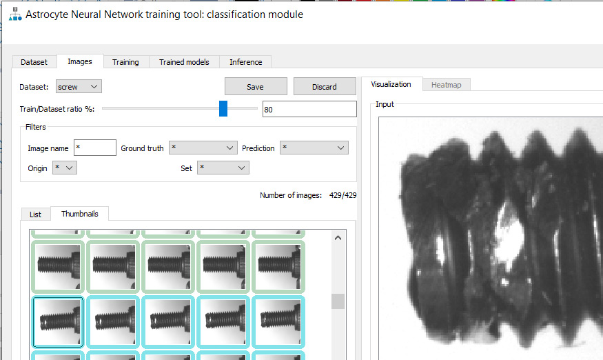
Figure 4 below illustrates classification training in Astrocyte where all samples are listed as thumbnails. For each sample, the rectangle around the thumbnail specifies the label (i.e., good or bad) and this information is editor by the user at training time. One easy way to automate this process is to put the samples in two different folders (good and bad) and use the folder names as labels. Another important aspect to consider when training a dataset is to reserve a portion of these samples for testing. One good rule in practice is to allocate 80% of the dataset for training while leaving the remaining 20% for testing, as seen in Figure 4 as the Train/Dataset Ratio %. When the training samples pass through the neural network, the weights of the neural network adjust for a certain number of iterations called epochs. Unlike training samples, testing samples are passed through the neural network for testing purposes without affecting the weights of the network. Training and testing groups of samples are important to develop a proper training model that will perform well in production.
Once the training set is created and labeled, the training process can begin. Training parameters are called Hyperparameters (as opposed to “parameters,” which are the actual weights of the neural network). Most common hyperparameters include the learning rate which tells the algorithm how fast to converge to a solution, the number of epochs which determines the number of iterations during the training process, the batch size which selects how many samples are processed at a time, and the model architecture that is selected to solve the problem. A common example of model architecture for a simple classification is ResNet, which is a Convolutional Neural Network, a frequently used model architecture in classification problems such as defect detection.
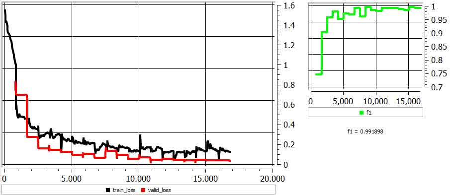
Once hyperparameters are configured (good training tools provide default values which work well in practice), the training process is ready to be launched. Training time ranges from a few minutes to a few hours and is dependent on the number of samples in your dataset, the hyperparameters, and the power/memory of your GPU card. During training, you can monitor two basic metrics: loss functions and accuracy. The loss functions show the difference between current model prediction (output of neural network) and expectation (the ground truth). These loss functions should go toward 0 while training. If they diverge, you may have to cancel the training session and restart it with different hyperparameters. The accuracy tells you how good your model is to properly classify samples. This metric should go toward 100% during training. In practice, you will rarely achieve 100% but often between 95% and 99%. Figure 5 depicts a graph of loss functions and accuracy while training in Astrocyte.
After training is complete with acceptable accuracy, your model is ready to use in production. Applying a model to real samples is called inference. Inference can be implemented on the PC using GPU cards or on an embedded device using a parallel processing engine. Depending on the size, weight, and power (SWAP) required by your application, various technologies are available for implementing deep learning on embedded devices such as GPUs, FPGAs and specialized neural processors.
Deep learning is more user-friendly and practical than ever before, enabling more applications to derive the benefits. Deep learning software has improved to the point that it can classify images better than any traditional algorithm—and may soon be able to outperform human inspectors.
 AI and medical imaging: building a relationship on solid data foundations
  A farewell to AI confusion