Bob’s Imaging Fundamentals #16: Scanning Electron Microscopes

Most of the time, Machine Vision applications count image acquisition times in the tens of milliseconds. For example, the frame time of an RS-170 camera at 30 frames per second is 1/30 = 0.0333 seconds (i.e. 33.33ms).  Of course, some Machine Vision engineers are ‘Type A’ personalities and feel the need to acquire images at much higher speed (e.g. Dalsa CA-D6 @ 955 fps! – 1/955 = 1.047ms/frame).  Well, more power to them and, after all, we’re going to need those guys when someone finally invents the Machine Vision X-Games, right?

Anyway, in applications where stuff zips by at a dizzying rate, the need for speed is an obvious one.  However, there are other areas of computer vision where images are acquired at extremely slow speeds.  I am speaking of course of Scanning Electron Microscopes, otherwise known as ‘SEM’.  Now before all you SEM experts start getting excited about all the mistakes I’m about to make in explaining SEM, rest assured, I have included a couple of links at the end of this article were people can go and find a decent explanation of them.

Basically, a SEM is a long upright tube with all the air sucked out.  At one end of the tube you have a device called an ‘Electron Gun’ that produces a stream of electrons and at the other end, you have a small ‘Sample Chamber’ housing a bunch of detectors.  In between the Electron Gun and the Sample Chamber is a series of magnetic doodads whose job it is to focus and direct the beam of electrons onto the object you want to image.  When the stream of electrons hits the object, electrons from the object itself break free and fly off in all directions inside the sample chamber.  Obviously, we don’t want all those electrons go to waste so we use the detectors in the sample chamber to ‘count’ the electrons that have broken free.  The more electrons hit the detectors the ‘brighter’ the object being bombarded with electrons.

Now the tricky question is how do we go from a beam firing electrons at object, to a recognizable image?  This is where the magnetic doodads come in; aside from making the electron beam tight and focused, they also allow us to aim the focused beam at specific points on the object.  Each time the beam is focused on a particular point of the object, electrons are fired for a predetermined amount of time then, the magnetic doodads move the beam to the next point and the electrons are fired again.  This process continues until a grid of points has been covered and the ‘brightness’ of each point in the grid has been evaluated.  In case you haven’t guessed by now, it’s this grid of points that gets turned into pixels and eventually an image.

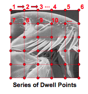
Obviously, the resolution of the final image will depend on how many scan points (also known as ‘dwell’ points) you have and how close together they are spaced; the closer your dwell points are to each other, the finer the details you can see on your object.  On the other hand, increasing the number of dwell points also means it take longer to build up your image because each dwell point takes a certain amount of time.  And there’s another problem, the electrons that have broken free of the object don’t all line up to get counted by the detectors.  In fact, when the focused electron beam hits the object, you’ve got electrons flying all over the place and if you don’t allow enough electrons to hit your detectors, the resulting image is fuzzy and grainy.  So how much time do we have to spend at each dwell point?  Good question.  Typically, SEM scan times are very slow in fact; they can vary from the 10’s of nanoseconds (i.e. 1/100ns = 10MHz) to the hundreds of microseconds (i.e. 1/100us = 10KHz).  In other words, if our dwell time is 100 microseconds and our image resolution is let’s say 640 x 480 dwell points, it will take roughly 30 seconds to capture the image (640 x 480 x 0.0001 seconds/point = 30.72 seconds).

Now here is where the Machine Vision bit comes in; if you happen to be putting your own SEM together and you are shopping around for a frame grabber to hook up to your electron counter thingy, the single most important thing you have to look out for is how low the frame grabber’s pixel clock can go.  Most of the time, frame grabbers are designed for pixel clocks that range in speeds from 10MHz to 40MHz (some even go as high as 120MHz).  But the fact is, very slow pixels clocks (e.g. 1 MHz or lower) can sometimes put you outside a frame grabber’s intend operating range.  So, if you want to grab from an SEM, be very sure of the frame grabber’s pixel clock specification before you lay down you hard earned money.

Helpful Links:

A College Level Explanation of SEM

An SEM explanation for the rest of us

Microscopy and Imaging resources on the web