From training to inference: Creating a neural network for image recognition
Graphical interfaces in Sapera and Astrocyte software make it easier to implement your own deep learning network
While traditional image processing software relies on task-specific algorithms, deep learning software uses a network to implement user-trained algorithms to recognize good and bad images or regions.
Fortunately, the advent of specialized algorithms and graphical user interface (GUI) tools for training neural networks is making it easier, quicker and more affordable for manufacturers. What can manufacturers expect from these deep-learning GUI tools and what’s it like using them?
Training: Creating the deep learning model
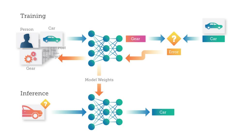
Training is the process of “teaching” a deep neural network (DNN) to perform a desired task — such as image classification or converting speech into text — by feeding it data that it can learn from. A DNN makes a prediction about what the data represents. Errors in the prediction are then fed back to the network to update the strength of the connections between the artificial neurons. The more data you feed the DNN, the more it learns, until the DNN is making predictions with a desired level of accuracy.
As an example, consider training a DNN designed to identify an image as being one of three different categories – a person, a car, or a mechanical gear.
Typically, the data scientist working with the DNN will have a previously-assembled training dataset, consisting of thousands of images, with each image labeled as a “person,” “car,” or “gear.” This could be an on-the-shelf dataset, such as Google’s Open Images, which includes nine million images, almost 60 million image-level labels, and much more.
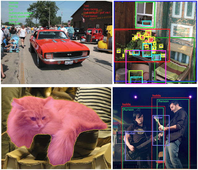
If the data scientist’s application is too specialized for an existing solution, then they may need to build their own training data set, collecting and labelling images that will best represent what the DNN needs to learn.
During the training process, as each image is passed to the DNN, the DNN makes a prediction (or inference) about what the image represents. Each error is fed back to the network to improve its accuracy in the next prediction.
Here the neural network predicts that one image of a “car” is a “gear.” This error is then propagated back through the DNN and the connections within the network are updated to correct for the error. The next time the same image is presented to the DNN, it will be more likely to make the correct prediction.

This training process continues with the images being fed to the DNN and the weights being updated to correct for errors, over and over again, dozens or thousands of times until the DNN is making predictions with the desired accuracy. At this point, the DNN is considered “trained” and the resulting model is ready to be used to categorize new images.
Right-sizing your neural network
The number of inputs, hidden layers, and outputs of a neural network is highly dependent on the problem you’re trying to solve and the particular design of your neural network. During the training process, a data scientist is trying to guide the DNN model to achieve a desired accuracy. This often requires running many, possibly hundreds of experiments, trying different DNN designs that vary by number of neurons and layers.
Between the input and output lay the neurons and connections of the network – the hidden layers. For many deep learning challenges, 1–5 layers of neurons are enough, since only a few features are being evaluated to make a prediction. But with more complex tasks, with more variables and considerations, you need more. Working with image or speech data may require a neural network of dozens to hundreds of layers, each performing a specific function, and millions or billions of weights connecting them.

Getting starting with sample collection
Traditionally, hundreds, or even thousands, of manually classified images were required to train the system and create a model that classifies objects with a high degree of predictability. But gathering and annotating such complex datasets has proven an obstacle to development, hindering deep learning adoption in mainstream vision systems.
Deep learning is well-suited to environments in which variables such as lighting, noise, shape, color and texture are common. A practical example that shows the strength of deep learning is scratch inspection on textured surfaces like brushed metal. Some scratches are less bright, with a contrast close to the textured background itself. Consequently, traditional techniques usually fail to reliably locate these types of defects, especially when the shape, brightness and contrast vary from sample to sample. Figure 1 illustrates scratch inspection on metal sheets. Defects are clearly shown via a heatmap image, which highlights the pixels at the location of the defect.
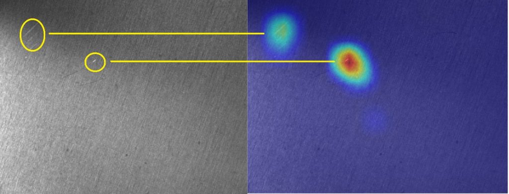
A deep neural network trained from scratch typically requires hundreds or even thousands of image samples. However, today’s deep learning software is often pre-trained, so users may only need tens of additional samples to adapt the system to their specific application.
In contrast, an inspection application built with regular classification would require the collection of both “good” and “bad” images for training. However, with new classification algorithms such as anomaly detection, users can train on good samples only and need only a few bad samples for final testing.
While there’s no magical way to collect image samples, it’s getting much easier. To collect images, technicians can use Sapera LT, a free image acquisition and control software development toolkit (SDK) for Teledyne DALSA’S 2D/3D cameras and frame grabbers. Astrocyte, a GUI tool for training neural networks, interfaces to Sapera LT to allow image collection from cameras. A user collecting images on PCB components in manual mode, for example, would move the PCB with their hands, changing the camera position, angle and distance to generate a series of views of the PCB components.
Training the neural network with visual tools
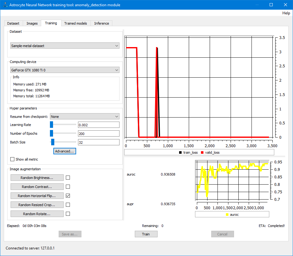
Once the user has the images, it’s time to train the neural network. Training is performed in Astrocyte by simply clicking on the “Train” button to start the training process with the default hyper-parameters. It’s possible to modify the hyper-parameters to achieve better accuracy on the final model.
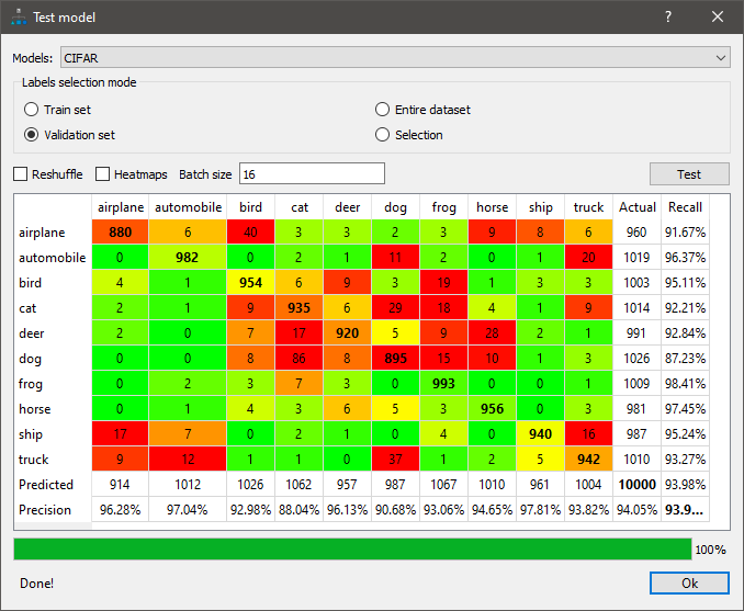
To verify accuracy, the user tests the model with a different set of images and may choose to employ diagnostic tools such as a confusion matrix for a classification model. A confusion matrix is a NxN table (where N = the number of classes) that shows the success rate for each class. In this example (see figure 2), color coding is used to represent the precision/recall success of the model, with green indicating a rate exceeding 90%.
Heatmaps are another critically important diagnostic tool. For example, when used in anomaly detection, a heatmap highlights the location of defects. When the user sees the heatmap, he/she assesses whether the image is good or bad for the right reasons. If the image was good but was classified as bad, the user can look at the heatmap for more detailed information. The neural network will follow what the user provided as input.
This usage of heatmaps on a screw-inspection application provides a good example:
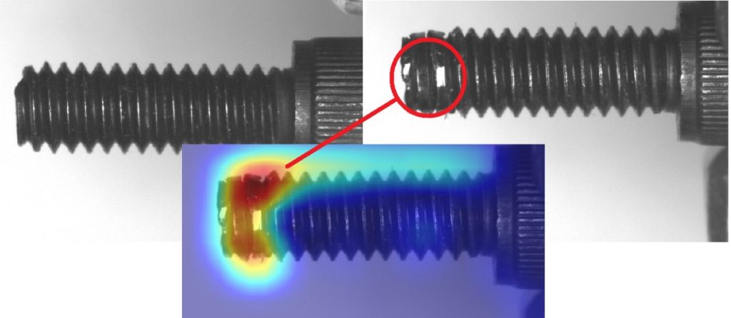
A heatmap can also reveal that a model is focusing on an image detail or feature that has no relevance to the desired analysis of the target scene or object in the image. Depending on the Astrocyte module, different types of heatmap-generation algorithms are available.
GUI tool in action
The best way to explain the GUI-tool approach to deep learning is to show it. Since anomaly detection model training is foundational to training neural networks, here’s a brief tutorial with a step-by-step approach to using Astrocyte for anomaly detection.
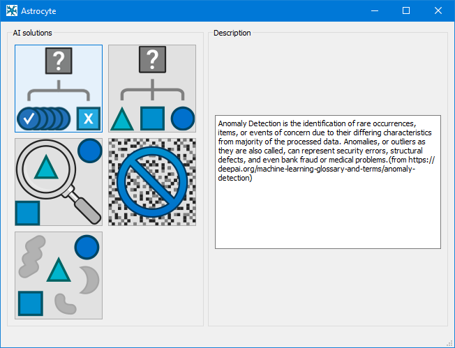
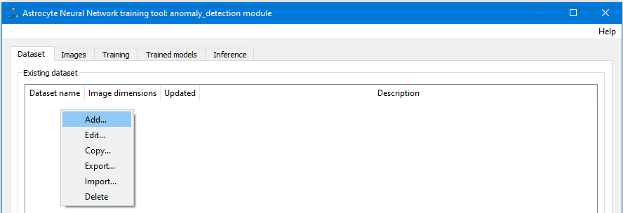
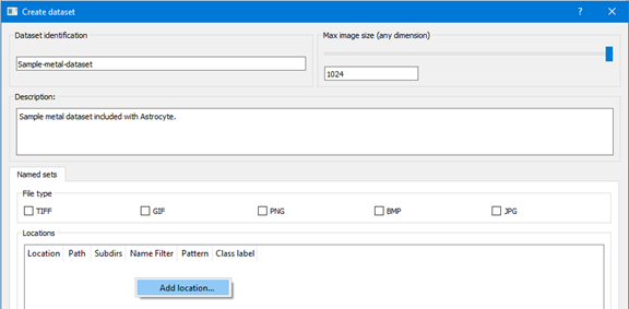
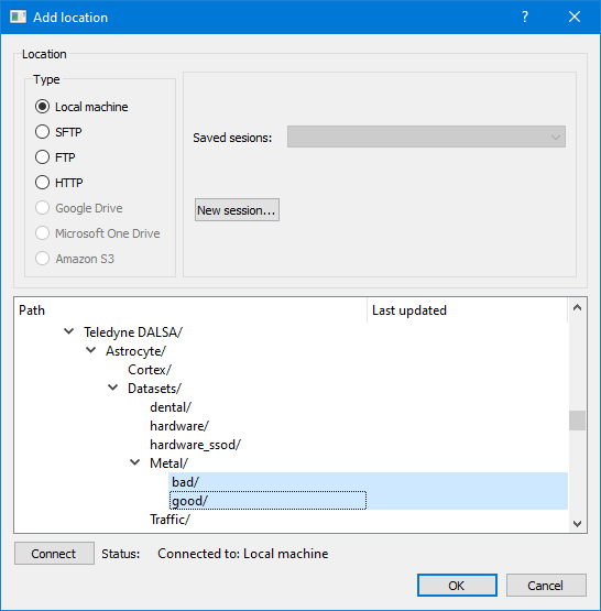
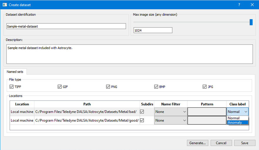
When the generation process is complete, the Image size distribution analyzer dialog is displayed if images in the dataset have varying sizes; otherwise, if images all have the same dimensions, they are automatically resized to the specified maximum image size and the dialog is not shown. If necessary, correct images using the Image Correction dialog.


Optimizing for inference: Do we need to refine our trainee?
Once the training portion is complete with acceptable accuracy, we end up with a weighted neural network — essentially a massive database. This is something that will work well, but perhaps is not optimal in terms of speed and power consumption. Some applications won’t tolerate high levels of latency: think intelligent transportation systems or even self-driving cars. Autonomous drones or other battery-powered systems might need to operate within a tight power envelope to meet flight time requirements.
The larger and more complex the DNN, the more compute, memory, and energy is consumed to both train it and run it. This may not work for your given application or device. In such cases, there is a desire to simplify the DNN after training to reduce power and latency, even if this simplification results in a slight reduction in prediction accuracy.
This kind of optimization is a relatively new area of deep learning. Chip and AI accelerator vendors typically create SDKs to help their users perform this kind of task – with software specifically tuned for their particular architectures. The chips involved can range widely, from GPUs, CPUs, FPGAs and neural processors. Each has its own advantages. For example, Nvidia’s TensorRT emphasize the company’s expertise in GPU cores. Xilink’s Vitis AI, in contrast, supports the company’s SoC like Versal including CPU, FPGA and neural processors.
Vendors typically offer variations on two types of approaches: pruning and quantization. Pruning is the action of removing parts of the neural network that have less of a contribution to the final result. This reduces the size/complexity of the network without significantly affecting the output precision. The second approach is quantization – reducing number of bits per weight (for example, replacing FP32 with FP16 or Quantized INT8/4/2). With less complex computation to perform, this can increase speed and/or reduce the hardware resources needed.
Ready for production: moving to inference
Once our DNN model is trained and optimized, it’s time to put it to work: making predictions against previously unseen data. This is like the training process, with images being fed as input, and the DNN attempting to classify it. Astrocyte.
Teledyne DALSA offers Sapera Processing and Sherlock, two software packages that feature a suite of image processing tools and an inference engine for running AI models built from
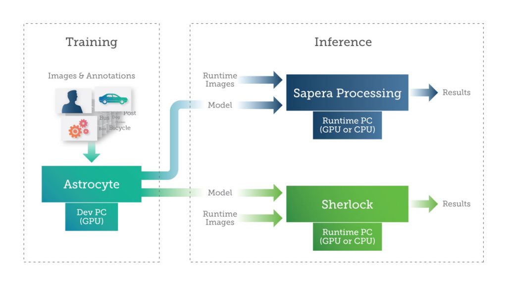
The user can implement inference on a PC using a GPU or CPU or on an embedded device. Depending on the size, weight and power (SWAP) requirements of the application, the user can leverage various technologies for implementing deep learning inference on embedded devices such as GPUs, FPGAs and specialized neural processors.
Deep Learning: easier every day?
At their heart, neural networks are complex and powerful tools. There are almost limitless opportunities to tweak and optimize each one to get the best performance for the problem you’re trying to solve. The sheer scope of optimization and the rapid pace of new research and tools can be overwhelming, even to seasoned practitioners.
But that doesn’t mean that you can’t start incorporating the benefits of these tools in your next vision system. The migration toward GUI tools is democratizing deep learning in vision systems. With software that frees users from the rigorous requirements of AI learning and programming experience, manufacturers are using deep learning to analyze images better than any traditional algorithm. And one day soon, such GUI tools may outperform any number of human inspectors.
Interested in learning more about deep-learning GUI tools for vision applications?
Watch this webinar or learn more about Teledyne DALSA Vision Software.


 AI & Embedded Vision — Driving System Innovation
  A farewell to AI confusion